What is Capital Budgeting: Its Importance, Techniques and Examples

1. What Is Capital Budgeting?

Capital budgeting, also called investment appraisal,  is the formal process by which a business evaluates potential major expenditures or investments. These are typically long-lived projects: purchasing new equipment, expanding into new markets, acquiring another company, constructing a facility, or launching a product line.

Unlike operational spending (day-to-day expenses), capital investments:

• Involve large sums of money committed upfront
• Generate returns over multiple years, often a decade or more
• Are difficult or impossible to reverse once initiated
• Directly shape a company’s competitive position and financial health

In short: Capital budgeting answers the question “Is this worth our money?”, and ensures that every dollar deployed creates more value than it costs.

2. How Capital Budgeting Works

At its core, capital budgeting revolves around one central idea: the time value of money. A dollar received today is worth more than a dollar received five years from now, because today’s dollar can be reinvested and earn returns.

The process involves:

1. Estimating cash flows — projecting the initial outlay (cash out) and the future cash inflows the project will generate
2. Applying a discount rate — typically the company’s Weighted Average Cost of Capital (WACC), to convert future cash flows into today’s dollars
3. Comparing results against predefined thresholds (hurdle rates, payback targets, or minimum acceptable returns)
4. Making a decision to accept, reject, or rank the investment among competing opportunities

The primary variables in any capital budgeting analysis are:

Variable	Description
Initial Investment (C₀)	Total upfront cost: equipment, installation, working capital changes
Operating Cash Flows (CF)	Net cash generated each period after taxes and expenses
Terminal Value	Salvage value or residual cash flows at project end
Discount Rate (r)	Cost of capital or required rate of return
Project Life (n)	Expected useful life of the investment in years

3. Why Capital Budgeting Matters

Capital budgeting is not just a financial exercise, it is a strategic imperative. Here is why businesses treat it as critical:

Risk Evaluation

Every major investment carries uncertainty. Capital budgeting provides structured tools , sensitivity analysis, scenario modeling, Monte Carlo simulation, to quantify risk, estimate the probability of unfavorable outcomes, and decide whether the expected return justifies exposure.

Optimal Resource Allocation

No company has unlimited capital. When multiple projects compete for the same pool of funds, capital budgeting provides objective ranking criteria, ensuring that resources flow toward the highest-value opportunities rather than pet projects or loudest advocates.

Strategic Alignment

Investments are not just about short-term returns, they define where a business is headed. A rigorous capital budgeting process filters out investments that may be profitable in isolation but misaligned with long-term strategy, preventing strategic drift.

Accountability and Performance Management

By establishing upfront financial projections and approval thresholds, capital budgeting creates a baseline against which actual performance can be measured. This closes the loop between planning and execution, making teams accountable for results.

Stakeholder Confidence

Boards, investors, and lenders look to capital budgeting as evidence that management makes disciplined, evidence-based investment decisions, particularly for large capital expenditure programs.

4. Objectives of Capital Budgeting

The main objectives of a sound capital budgeting framework are:

• Maximize shareholder value by directing capital into projects that generate returns above the cost of capital
• Achieve optimal resource allocation by systematically comparing competing investment opportunities
• Ensure long-term financial stability by assessing the future cash flow profile of proposed investments and their impact on liquidity
• Manage risk by identifying, quantifying, and mitigating the uncertainties inherent in long-term projects
• Support strategic execution by ensuring that capital deployment aligns with corporate goals, competitive positioning, and growth plans

5. The Capital Budgeting Process — Step by Step

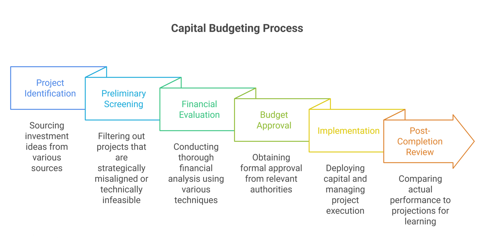
Step 1: Project Identification

The process begins with sourcing investment ideas. These may come from:

• Internal teams identifying operational bottlenecks that new equipment could resolve
• Market research revealing unmet customer needs
• Strategic planning sessions uncovering adjacencies for expansion
• Competitive intelligence flagging threats that require a defensive investment

The goal at this stage is to build a pipeline of candidate projects aligned with the company’s strategic direction.

Step 2: Preliminary Screening

Not every idea warrants full-scale financial analysis. A first filter screens out projects that are:

• Strategically misaligned
• Technically infeasible given current capabilities
• Clearly below the company’s minimum return threshold based on rough estimates

This stage saves significant analytical resources by narrowing the field before deep-dive evaluation begins.

Step 3: Financial Evaluation

For projects that pass screening, a thorough financial analysis is conducted. This involves:

• Estimating incremental cash flows — not accounting profits, but actual cash generated by the project net of taxes
• Determining the appropriate discount rate — usually WACC, adjusted for project-specific risk
• Applying one or more capital budgeting techniques (NPV, IRR, Payback Period, etc.)
• Performing sensitivity analysis to understand how results change under different assumptions
• Modeling scenarios — base case, optimistic, and pessimistic — to bound the range of possible outcomes

Step 4: Budget Approval

Projects that clear the financial evaluation move to formal approval. Depending on investment size:

• Small projects may be approved at the department or business unit level
• Medium projects require CFO or executive committee sign-off
• Large projects require board of directors approval

The approval process considers not just financial metrics but also strategic fit, management capacity to execute, and financing availability.

Step 5: Implementation

With approval granted, capital is deployed. This phase involves:

• Procurement of assets, services, or technology
• Project management to keep the initiative on time and on budget
• Change management to handle organizational impacts
• Tracking of actual cash flows against projected figures

Step 6: Post-Completion Review (Performance Audit)

Often overlooked, this final step is critical for organizational learning. After a project is operational, actual performance is compared to the initial projections used for approval. Key questions:

• Did the project deliver the projected cash flows?
• Were there cost overruns or timeline delays?
• What assumptions proved wrong, and why?
• What can be applied to improve future capital budgeting analyses?

Post-completion reviews create a virtuous cycle of continuous improvement in investment decision-making.

6. Types of Capital Investment Decisions

Capital budgeting covers a wide variety of investment categories:

Investment Type	Examples
Expansion	Opening new locations, entering new markets, adding production capacity
Replacement	Swapping aging or obsolete equipment for modern, more efficient alternatives
New Product / Service	R&D investment, product development, service innovation
Cost Reduction	Automation, process re-engineering, technology upgrades to lower operating costs
Regulatory / Compliance	Environmental controls, safety systems, legal mandates (these may have no direct financial return but are unavoidable)
Strategic / Defensive	Acquisitions, intellectual property investments, investments to block competitor entry

7. Capital Budgeting Techniques and Methods

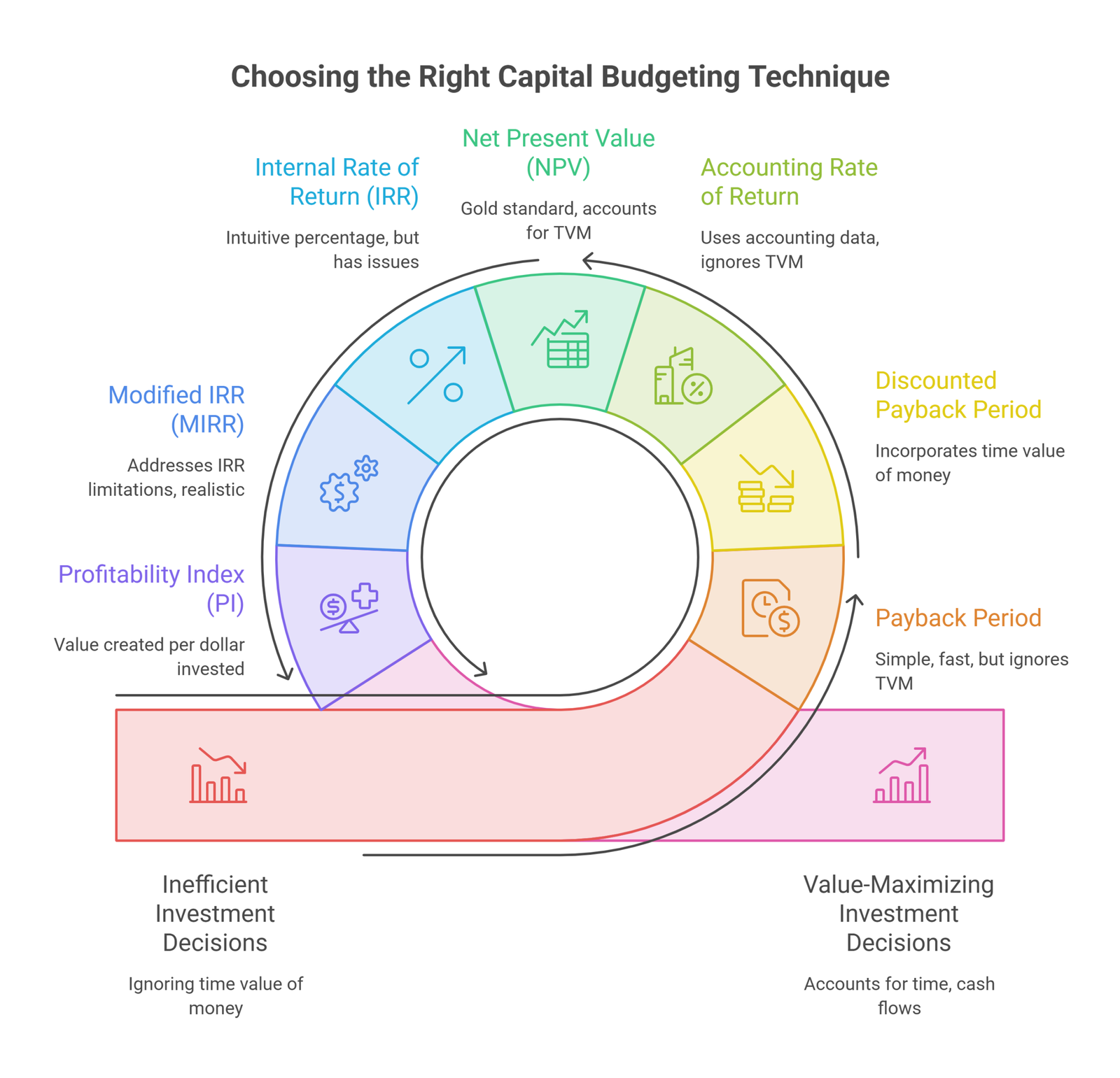
Capital budgeting offers a toolkit of evaluation methods. The most widely used are:

7.1 Payback Period

What it measures: How long it takes for a project’s cumulative cash inflows to recover the initial investment.

Formula:

Payback Period = Initial Investment ÷ Annual Net Cash Inflow

For uneven cash flows:

Payback Period = Year before full recovery + (Remaining balance ÷ Cash flow in recovery year)

Example:

• Initial investment: $500,000
• Annual cash inflows: $125,000
• Payback Period = $500,000 ÷ $125,000 = 4 years

Decision rule: Accept if payback period ≤ company’s maximum acceptable payback period.

Pros:

• Simple and fast to calculate
• Easy for non-financial stakeholders to understand
• Useful for companies with liquidity concerns or high-uncertainty environments
• Good first-pass screen for obvious non-starters

Cons:

• Ignores time value of money
• Ignores cash flows after the payback period (a project with a 5-year payback might generate 20 years of cash flows)
• Can lead to rejecting long-term, high-value investments in favor of quick-return but lower-value projects

7.2 Discounted Payback Period

An enhancement of the simple payback period that discounts cash flows before calculating recovery time, incorporating the time value of money.

Formula: Same as payback period but applied to discounted (present value) cash flows.

Why it matters: Gives a more conservative and realistic view of how long it actually takes, in economic terms, to recover an investment.

7.3 Accounting Rate of Return (ARR)

What it measures: The average annual accounting profit generated by a project, expressed as a percentage of the initial (or average) investment.

Formula:

ARR = (Average Annual Net Profit ÷ Initial Investment) × 100

Example:

• Project cost: $200,000
• Average annual profit after depreciation and taxes: $30,000
• ARR = ($30,000 ÷ $200,000) × 100 = 15%

Decision rule: Accept if ARR ≥ target accounting return.

Pros:

• Uses readily available accounting data
• Considers the project’s full lifespan
• Intuitive percentage format familiar to non-financial managers

Cons:

• Based on accounting profit, not cash flows
• Ignores time value of money
• Can be distorted by accounting choices (depreciation method, asset write-downs, etc.)

7.4 Net Present Value (NPV)

The gold standard of capital budgeting. NPV calculates the value created by a project in today’s dollars by discounting all future cash flows at the company’s required rate of return and subtracting the initial investment.

Formula:

NPV = Σ [CFₜ ÷ (1 + r)ᵗ] − C₀

Where:

• CFₜ = Net cash flow in period t
• r = Discount rate (cost of capital / hurdle rate)
• t = Time period
• C₀ = Initial investment (at t = 0)

Example:

• Initial investment: $1,000,000
• Discount rate: 10%
• Cash flows: $300,000 (Y1), $350,000 (Y2), $400,000 (Y3), $350,000 (Y4), $300,000 (Y5)

Year	Cash Flow	PV Factor (10%)	Present Value
1	$300,000	0.9091	$272,730
2	$350,000	0.8264	$289,240
3	$400,000	0.7513	$300,520
4	$350,000	0.6830	$239,050
5	$300,000	0.6209	$186,270
Total PV			$1,287,810
Less: Initial Investment			$1,000,000
NPV			$287,810

A positive NPV of $287,810 means the project is expected to create $287,810 of value above and beyond the cost of capital.

Decision rule:

• NPV > 0 → Accept (value-creating)
• NPV < 0 → Reject (value-destroying)
• NPV = 0 → Indifferent (earns exactly the required return)
• For mutually exclusive projects: choose the highest NPV

Pros:

• Accounts for time value of money
• Measures absolute value creation in dollar terms
• Theoretically consistent — maximizing NPV maximizes shareholder wealth
• Handles unconventional cash flow patterns correctly

Cons:

• Requires an accurate estimate of the discount rate, which can be challenging
• Can favor larger projects over smaller, more capital-efficient ones (this is where PI helps)
• Does not convey the return as a percentage (managers often prefer a rate metric alongside NPV)

7.5 Internal Rate of Return (IRR)

What it measures: The discount rate at which the NPV of a project equals exactly zero, in other words, the effective annual return generated by the investment.

Formula: Solve for r in:

0 = Σ [CFₜ ÷ (1 + r)ᵗ] − C₀

This cannot be solved algebraically for complex cash flows and requires iterative calculation (Excel’s IRR() function handles this automatically).

Example (using the same project above): The IRR would be approximately 24.9% — meaning the project generates a ~25% annual return on the invested capital.

Decision rule:

• IRR > Cost of capital (hurdle rate) → Accept
• IRR < Cost of capital → Reject
• For mutually exclusive projects: choose the highest IRR (with caution — see limitations)

Pros:

• Intuitive percentage format easy to communicate to non-financial stakeholders
• Directly comparable to the company’s hurdle rate or cost of capital
• Popular in practice for its clarity and ease of communication

Cons:

• Multiple IRR problem: Projects with non-conventional cash flows (multiple sign changes) can have multiple IRRs, making the result ambiguous
• Reinvestment rate assumption: IRR implicitly assumes cash flows are reinvested at the IRR itself, which is often unrealistic
• Scale problem: A smaller project with a 40% IRR may have a lower NPV than a larger project with a 20% IRR — IRR alone can mislead when comparing projects of different sizes
• Conflict with NPV: For mutually exclusive projects, IRR and NPV rankings can diverge — when they do, NPV is the theoretically correct criterion

7.6 Modified Internal Rate of Return (MIRR)

What it addresses: The key limitations of IRR — specifically the unrealistic reinvestment rate assumption and the multiple IRR problem.

How it works: MIRR calculates a single rate of return by:

1. Discounting negative cash flows (outflows) to the present at the financing rate (cost of capital)
2. Compounding positive cash flows (inflows) to the end of the project at the reinvestment rate (typically the cost of capital or the market rate)
3. Solving for the rate that equates these terminal values

Formula:

MIRR = [(FV of positive cash flows at reinvestment rate) ÷ (PV of negative cash flows at financing rate)]^(1/n) − 1

Advantages over IRR:

• Produces only one rate (eliminates multiple IRR problem)
• More realistic reinvestment assumption
• Consistent with NPV rankings for mutually exclusive projects

7.7 Profitability Index (PI)

What it measures: The ratio of the present value of future cash flows to the initial investment — or the value created per dollar invested.

Formula:

PI = Present Value of Future Cash Flows ÷ Initial Investment

Or equivalently:

PI = (NPV + Initial Investment) ÷ Initial Investment = 1 + (NPV ÷ Initial Investment)

Using the earlier example:

• PV of cash flows: $1,287,810
• Initial investment: $1,000,000
• PI = 1.29

Decision rule:

• PI > 1.0 → Accept (creates value)
• PI < 1.0 → Reject (destroys value)
• PI = 1.0 → Indifferent

When PI is especially useful: Capital rationing — when a company must allocate a fixed capital budget across multiple projects, ranking by PI identifies the combination of projects that maximizes total value per dollar spent.

8. Technique Comparison Table

Technique	Time Value of Money	Measures	Best Used For	Key Limitation
Payback Period	✗ No	Liquidity / speed of recovery	Quick screening; liquidity-constrained firms	Ignores post-payback cash flows
Discounted Payback	✓ Yes	Risk-adjusted liquidity	Firms combining time-value rigor with liquidity focus	Still ignores post-payback cash flows
ARR	✗ No	Accounting profitability %	Targets tied to accounting metrics	Based on profits, not cash flows
NPV	✓ Yes	Absolute value created ($)	Primary decision criterion	Requires accurate discount rate
IRR	✓ Yes	Percentage return	Communicating returns; comparing to hurdle rate	Multiple IRRs; scale problem
MIRR	✓ Yes	Realistic % return	Overcoming IRR’s limitations	Less widely known/understood
PI	✓ Yes	Value per dollar invested	Capital rationing; ranking under budget constraint	Doesn’t show absolute value

Best practice: Use NPV as the primary criterion, supported by IRR (or MIRR) for communication, and PI when capital is rationed.

9. Real-World Example: A Full Capital Budgeting Analysis

Scenario: EcoTech Manufacturing — Automated Production Line

Background: EcoTech is a mid-sized manufacturer of industrial components. Management is evaluating a $2 million automated production line that would replace manual processes, reduce per-unit costs, and increase output capacity. The company’s cost of capital (WACC) is 12%, and the machine has a projected useful life of 6 years, after which it can be sold for an estimated $150,000 salvage value.

Projected Cash Flows:

Year	Incremental Revenue	Cost Savings	Operating Expenses	Taxes (30%)	Net Cash Flow
0	—	—	—	—	−$2,000,000
1	$400,000	$250,000	$80,000	$171,000	$399,000
2	$420,000	$260,000	$82,000	$179,400	$418,600
3	$440,000	$270,000	$84,000	$187,800	$438,200
4	$460,000	$275,000	$86,000	$194,700	$454,300
5	$480,000	$280,000	$88,000	$201,600	$470,400
6	$500,000	$285,000	$90,000	$208,500 + $150,000 salvage	$636,500

Step 1 — Payback Period:

Year	Net Cash Flow	Cumulative Cash Flow
1	$399,000	$399,000
2	$418,600	$817,600
3	$438,200	$1,255,800
4	$454,300	$1,710,100
5	$470,400	$2,180,500 ✓

Payback Period = 4 + ($2,000,000 − $1,710,100) / $470,400 = 4.62 years

Step 2 — NPV Calculation at 12%:

Year	Cash Flow	PV Factor (12%)	PV of Cash Flow
1	$399,000	0.8929	$356,268
2	$418,600	0.7972	$333,707
3	$438,200	0.7118	$311,893
4	$454,300	0.6355	$288,700
5	$470,400	0.5674	$266,866
6	$636,500	0.5066	$322,450
Total PV			$1,879,884

NPV = $1,879,884 − $2,000,000 = −$120,116

At 12% discount rate, the NPV is slightly negative.

Step 3 — IRR: By iteration, the IRR ≈ 10.6% — below the 12% hurdle rate, consistent with the negative NPV.

Step 4 — Profitability Index: PI = $1,879,884 / $2,000,000 = 0.94 (below 1.0 — confirm rejection)

Decision: Under current assumptions, the project does not meet EcoTech’s required 12% return. However, management should conduct sensitivity analysis:

• If cost savings increase by 10%, does the project become NPV-positive?
• What if the salvage value is $250,000 instead of $150,000?
• At what discount rate (i.e., if WACC changes) does the project become viable?

This kind of scenario analysis transforms a binary accept/reject into a strategic conversation about assumptions, risks, and value levers.

10. Real-World Case Studies from Leading Companies

Tesla — Gigafactory

Tesla’s Gigafactory in Nevada stands as one of the most ambitious capital budgeting decisions in modern manufacturing history. Tesla used discounted cash flow methods to evaluate the initial multi-billion-dollar investment, projecting that the Gigafactory would reduce battery costs by up to 30% while increasing production capacity tenfold. The analysis weighed not only financial returns but also strategic outcomes — securing battery supply, lowering vehicle costs, and accelerating market penetration. The Gigafactory also incorporated non-financial factors: carbon footprint, community development, and job creation. This exemplifies modern capital budgeting, where quantitative financial analysis is embedded within a broader strategic and ESG-aware framework.

Amazon — Logistics Network Expansion

Amazon’s sustained investment in building one of the world’s most sophisticated logistics networks — warehouses, last-mile delivery infrastructure, robotics — is a multi-decade capital budgeting story. The financial justification went beyond direct margin improvement: Amazon modeled the network effect, where faster delivery times increase conversion rates, reduce customer acquisition costs, and deepen Prime membership lock-in. This illustrates a critical advanced capital budgeting concept — externalities and interdependencies between projects, where the full value of an investment is only realized when viewed within the broader portfolio context.

Apple — Research and Development Investment

Apple’s consistent allocation of large capital budgets to R&D — and its careful evaluation of which technologies and form factors to commercialize — demonstrates capital budgeting at a product-portfolio level. Apple famously killed projects (like the original Newton) when financial analysis showed they would not achieve the required scale of return, and invested aggressively when proprietary technology (like the A-series chip) promised a durable competitive moat. The lesson: capital budgeting is not just about approving investments — it is equally about disciplined rejection.

11. Advantages and Limitations

Advantages

• Rigor before commitment: Thorough financial analysis prevents impulsive or politically-motivated investment decisions, replacing intuition with data.
• Objective comparison: Multiple competing projects can be ranked using consistent, comparable metrics, ensuring the best opportunities rise to the top.
• Long-term focus: Capital budgeting forces managers to think in multi-year cash flow terms, counteracting short-termism driven by quarterly earnings pressure.
• Risk quantification: Sensitivity analysis and scenario modeling surface risks early, when they can still be managed or mitigated.
• Strategic alignment: The formal approval process ensures investments support declared corporate strategy, not departmental agendas.
• Accountability: Projected cash flows create a benchmark for post-implementation performance review.

Limitations

• Forecast uncertainty: All capital budgeting techniques depend on projected future cash flows, which are inherently uncertain. Garbage in, garbage out — poor assumptions produce misleading outputs regardless of analytical sophistication.
• Discount rate sensitivity: NPV and IRR results can shift dramatically with small changes in the discount rate. Determining the correct rate — especially for projects with unusual risk profiles — is more art than science.
• Ignores qualitative factors: Quantitative models struggle to capture strategic optionality, brand value, employee morale, or competitive signaling — all of which may be decisive in a real investment decision.
• Short payback bias: Companies relying heavily on payback period metrics may systematically underinvest in long-duration, high-value projects (infrastructure, R&D, brand-building).
• Static analysis in a dynamic world: Most capital budgeting models assume a fixed project life and predetermined cash flows. They do not naturally capture management’s ability to adjust, expand, contract, or abandon a project in response to new information — an issue that real options analysis attempts to address.
• Gaming and optimism bias: In organizations where capital allocation is competitive, project sponsors may systematically overestimate returns or underestimate costs to win approval. Post-completion reviews are the primary check on this behavior.

12. Capital Budgeting Best Practices

1. Use Multiple Techniques in Combination

No single technique is perfect. The recommended approach:

• NPV as the primary decision criterion (measures absolute value creation)
• IRR or MIRR for intuitive communication with non-financial stakeholders
• Payback Period as a risk and liquidity filter
• PI for capital rationing decisions

2. Conduct Rigorous Sensitivity Analysis

Identify the key assumptions driving the analysis, typically volume, pricing, costs, and timing, and test how NPV and IRR change when those assumptions vary. A project that looks attractive under base-case assumptions but collapses under mild adverse conditions may warrant caution or require risk mitigation before proceeding.

3. Apply Scenario Analysis

Go beyond single-point estimates. Model:

• Base case: Most likely outcome
• Optimistic case: Upside scenario (favorable market, cost efficiencies)
• Pessimistic case: Downside scenario (lower revenues, cost overruns, delays)

This gives decision-makers a probability-weighted sense of expected value and worst-case exposure.

4. Match the Discount Rate to Project Risk

The WACC is a good default discount rate, but individual projects may carry more or less risk than the company average. High-risk projects (new markets, unproven technology) warrant a higher discount rate. Low-risk projects (regulatory compliance, maintenance replacements) may use a lower rate. Using a single WACC for all projects can lead to under-investment in low-risk opportunities and over-investment in high-risk ones.

5. Involve Cross-Functional Stakeholders

Financial analysis is only as good as its underlying assumptions. Bringing in operations, sales, engineering, and supply chain teams improves estimate quality, surfaces hidden risks, and increases organizational commitment to the approved project.

6. Conduct Disciplined Post-Completion Reviews

Track actual versus projected performance for every major project. Share findings across the organization. This closes the feedback loop, improves future forecasting quality, and holds project sponsors accountable.

7. Consider Real Options Value

Some investments create strategic flexibility that pure DCF analysis undervalues. A pilot program that could be scaled if successful has embedded option value. An investment in a platform technology may enable future product lines not yet identified. Where such options are material, supplement NPV analysis with a qualitative or quantitative assessment of the optionality.

13. Key Metrics Quick Reference

Metric	Formula	Decision Rule	Best For
Payback Period	Initial Investment ÷ Annual CF	Accept if ≤ target payback	Liquidity assessment
ARR	(Avg. Net Profit ÷ Initial Investment) × 100	Accept if ≥ target ARR	Accounting-based evaluation
NPV	Σ [CFₜ / (1+r)ᵗ] − C₀	Accept if NPV > 0	Primary decision criterion
IRR	Rate where NPV = 0	Accept if IRR > hurdle rate	Communicating % returns
MIRR	[(FV positive CFs ÷ PV negative CFs)^(1/n)] − 1	Accept if MIRR > hurdle rate	Replacing IRR’s limitations
PI	PV of CFs ÷ Initial Investment	Accept if PI > 1.0	Capital rationing

Frequently Asked Questions

What is the difference between capital budgeting and operational budgeting? 

Operational budgets cover day-to-day expenses of running the business (salaries, utilities, supplies). Capital budgets cover long-term investments in assets expected to deliver value over multiple years. The two are complementary: capital investments often create the capacity that operational budgets fund to run.

Which capital budgeting technique is best?

NPV is the theoretically superior method because it directly measures value creation in absolute dollar terms and accounts for the time value of money. However, in practice, companies typically use NPV alongside IRR (for intuitive communication) and payback period (for liquidity and risk assessment).

What is a hurdle rate? 

A hurdle rate is the minimum acceptable rate of return a project must clear to be approved. It is typically set at the company’s WACC, sometimes with a premium added for specific risk factors. Projects with IRRs below the hurdle rate are expected to destroy value.

How does capital budgeting differ for small businesses versus large corporations? 

The principles are identical, but scale and formality differ. Large corporations maintain dedicated capital planning teams, formal approval committees, and sophisticated modeling tools. Small businesses may conduct the same analysis in a spreadsheet with a single decision-maker. The rigor of the analysis should be proportional to the size and reversibility of the investment.

What is capital rationing? 

Capital rationing occurs when a company has more value-creating investment opportunities than available capital. The solution is to rank projects by Profitability Index (PI) and fund from the top down until the capital budget is exhausted.

Conclusion

Capital budgeting is one of the most consequential activities in corporate finance. The decisions made through this process, which factories to build, which technologies to bet on, which markets to enter, define a company’s trajectory for years or even decades.

Done well, capital budgeting ensures that every dollar of scarce capital is deployed where it creates the greatest long-term value. It replaces gut instinct with evidence, surfaces risks before they become losses, and aligns investment decisions with strategic intent.

The toolkit is powerful: NPV measures absolute value creation. IRR communicates returns in intuitive percentage terms. Payback Period screens for liquidity risk. PI enables rational prioritization under capital constraints. MIRR corrects IRR’s most problematic assumptions. Used in combination, supported by sensitivity analysis, scenario planning, and post-completion review, these techniques form a complete system for disciplined long-term investment decision-making.

Whether evaluating a $50,000 equipment replacement or a $5 billion facility expansion, the underlying logic is the same: invest when the expected return exceeds the cost, and let the numbers,  rigorously derived,  guide the decision.

Are your long-term investments backed by rock-solid data, or just gut instinct? Whether you’re greenlighting a major expansion, upgrading equipment, or launching a new product line, a guessing game can cost millions. Oak Business Consultant provides expert Financial Modeling services to take the risk out of your capital budgeting. We build custom, rigorous NPV, IRR, and sensitivity analysis models to ensure every dollar you deploy maximizes shareholder value and drives strategic growth. Schedule your free capital budgeting consultation.