Top 10 Formulas For Your Financial Model In Excel

Top 10 Excel Formulas for Financial Modeling, with Examples

Most broken financial models do not fail on hard maths. They fail on small things: a lookup that returns the wrong row, a loan payment that forgot to divide the rate by 12, or an NPV that discounts the opening investment by a year.

Audits of 54 real spreadsheets published since 1997 found errors in 91% of them, according to research by Raymond Panko at the University of Hawaii. Using a short list of formulas well is the cheapest fix.

This guide covers ten formulas that do most of the work in a financial model in Excel. Each one has its syntax, a worked example with real numbers, and the mistake it invites most often.

The ten formulas at a glance

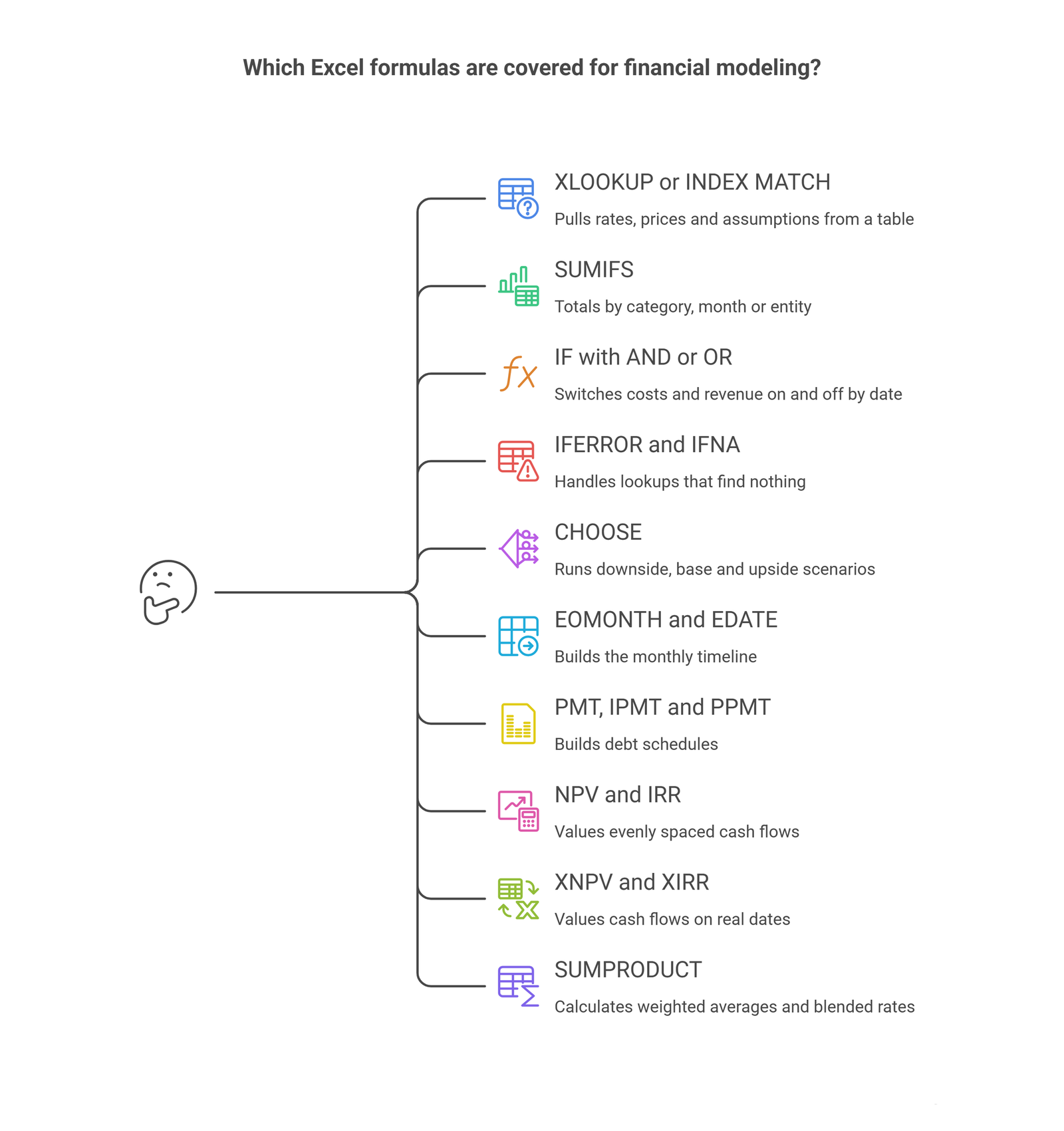
#	Formula	What it does in a model	Excel version
1	XLOOKUP or INDEX MATCH	Pulls rates, prices and assumptions from a table	XLOOKUP needs Microsoft 365 or Excel 2021 and later
2	SUMIFS	Totals by category, month or entity	All versions
3	IF with AND or OR	Switches costs and revenue on and off by date	All versions
4	IFERROR and IFNA	Handles lookups that find nothing	All versions
5	CHOOSE	Runs downside, base and upside scenarios	All versions
6	EOMONTH and EDATE	Builds the monthly timeline	All versions
7	PMT, IPMT and PPMT	Builds debt schedules	All versions
8	NPV and IRR	Values evenly spaced cash flows	All versions
9	XNPV and XIRR	Values cash flows on real dates	All versions
10	SUMPRODUCT	Calculates weighted averages and blended rates	All versions

1. XLOOKUP and INDEX MATCH

Lookups connect the inputs sheet to the calculations. A tax rate, a price list or a salary band sits in one table and feeds many cells.

=XLOOKUP(lookup_value, lookup_array, return_array, [if_not_found], [match_mode], [search_mode])

=XLOOKUP(B5, Inputs!A:A, Inputs!C:C, “Missing”)

XLOOKUP matches exactly by default and can return a value from a column to the left of the lookup column. Microsoft announced it in 2019 as the successor to VLOOKUP.

Excel 2019 and earlier show #NAME? when they meet XLOOKUP. If the file goes to someone on an older version, use INDEX MATCH instead.

=INDEX(Inputs!C:C, MATCH(B5, Inputs!A:A, 0))

The 0 forces an exact match. The common mistake is VLOOKUP with the last argument left blank. Excel then uses approximate matching and can return the wrong row without any warning.

2. SUMIFS

SUMIFS adds values that meet one or more conditions. It turns a transaction list into monthly and category totals.

=SUMIFS(sum_range, criteria_range1, criteria1, [criteria_range2, criteria2], …)

Take five rows of data: Jan Software 18,000, Jan Services 12,000, Feb Software 21,000, Feb Services 9,500 and Mar Software 19,500. Months sit in A2:A6, product lines in B2:B6 and revenue in C2:C6.

=SUMIFS(C2:C6, B2:B6, “Software”, A2:A6, “Feb”)

This returns 21,000. Software across all three months returns 58,500. Point the criteria at cells, not typed text, so one change updates every total. Note that SUMIFS puts the sum range first, while the older SUMIF puts it last.

3. IF with AND or OR

IF tests a condition and returns one value if true and another if false. In a model, it usually controls timing: when a hire starts, when a contract ends, when a loan is drawn.

=IF(AND(F3>=C5, F3<=D5), $E5, 0)

Here F3 holds the month-end date, C5 the start date, D5 the end date and E5 the monthly cost. The contractor is paid only between the two dates. Without AND, this needs two nested IFs.

Deep nesting is the usual failure. Past three levels, switch to IFS or build a 1/0 flag row and multiply by it.

4. IFERROR and IFNA

A lookup that finds nothing returns #N/A, and one error can spread through a whole sheet. IFERROR replaces it with a value you choose.

=IFERROR(XLOOKUP(B5, Inputs!A:A, Inputs!C:C), 0)

Use it sparingly. A silent zero can hide a broken link or a misspelled name. Wrap only the lookup, never a whole calculation. If #N/A is the only error you expect, use IFNA, which ignores every other error type.

Add one check cell that counts errors in the sheet. For example, =SUMPRODUCT(–ISERROR(C5:C200)) should always show 0.

5. CHOOSE

CHOOSE returns the nth value from a list. It is the simplest scenario switch in Excel.

=CHOOSE(index_num, value1, value2, value3)

=CHOOSE(C2, F10, G10, H10)

Cell C2 holds 1 for downside, 2 for base or 3 for upside. F10:H10 hold growth rates of 4%, 8% and 12%. With C2 set to 2, growth is 8%, and year-one revenue on a 500,000 base is 540,000.

Keep the scenario values in cells, not typed inside the formula. That way a reviewer can see and change every assumption in one place.

6. EOMONTH and EDATE

Nearly every model runs on a timeline. EOMONTH returns the last day of a month, a set number of months away. EDATE keeps the same day of the month.

=EOMONTH(start_date, months)

=EOMONTH(DATE(2026,1,1), 0)

=EOMONTH(C3, 1)

The first formula returns 31 Jan 2026. The second, copied across the row, returns 28 Feb 2026, then 31 Mar 2026, and so on. Typing each date by hand is the mistake to avoid, because one typo shifts every period after it.

Use EDATE for events that fall on a fixed day. =EDATE(DATE(2026,1,15), 1) returns 15 Feb 2026, which suits invoice and repayment dates.

7. PMT, IPMT and PPMT

These three build a debt schedule. PMT gives the level payment. IPMT and PPMT split a given payment into interest and principal.

=PMT(rate, nper, pv, [fv], [type])

=PMT(8%/12, 60, -250000)

For a 250,000 loan at 8% over five years with monthly payments, PMT returns 5,069.10. Month one then splits into 1,666.67 of interest from =IPMT(8%/12, 1, 60, -250000) and 3,402.43 of principal from =PPMT(8%/12, 1, 60, -250000). The two add up to the payment.

The classic error is feeding an annual rate into a monthly schedule. Divide the rate by 12 and count periods in months. Enter the loan as a negative number if you want a positive payment.

8. NPV and IRR

NPV discounts a series of cash flows to today. IRR finds the discount rate at which that value is zero. Both assume the cash flows arrive at equal intervals.

Say the opening outlay of -120,000 sits in B3. Five yearly inflows of 30,000, 40,000, 50,000, 45,000 and 35,000 sit in C3:G3. The discount rate is 10%.

=NPV(10%, C3:G3) + B3

=IRR(B3:G3)

NPV returns 30,364.17 and IRR returns 19.08%. Oak’s NPV calculator can confirm the same result.

The mistake that catches people is including the outlay inside the function. =NPV(10%, B3:G3) returns 27,603.79, because NPV treats the first value as arriving one period from now. Add the outlay outside the function, as above.

9. XNPV and XIRR

Real cash flows rarely arrive on neat anniversaries. XNPV and XIRR use actual dates, so they suit project and investment cases in a DCF model.

=XNPV(rate, values, dates)

=XIRR(values, dates, [guess])

Take the same project with dated flows: -120,000 on 1 Jan 2026, then 30,000 on 30 Jun 2026, 40,000 on 15 Mar 2027, 50,000 on 31 Dec 2027 and 60,000 on 30 Sep 2028. At 10%, XNPV returns 31,807.65 and XIRR returns 26.25%.

Two differences from NPV matter. XNPV includes the first value inside the function and does not discount it. And both functions need real date values, not text that looks like dates. XIRR also needs at least one positive and one negative cash flow.

10. SUMPRODUCT

SUMPRODUCT multiplies matching cells in two or more ranges, then adds the results. In a model, it is the standard way to get a weighted average.

=SUMPRODUCT(B2:B4, C2:C4) / SUM(B2:B4)

Three products earn revenue of 120,000, 80,000 and 50,000, at gross margins of 40%, 25% and 55%. The formula returns a blended margin of 38.2%. A plain AVERAGE of the three margins gives 40%, which overstates profit because it ignores the weights.

Ranges must be the same size, or SUMPRODUCT returns #VALUE!. Text inside a range counts as zero.

Formulas to use less

Four habits cause trouble in larger models.

• VLOOKUP. It works, but the column number is typed by hand. Insert a column and the formula quietly points at the wrong one.
• OFFSET and INDIRECT. Both are volatile, like NOW, TODAY and RAND. Excel recalculates them on almost every change, along with everything downstream. Chandoo’s guide to volatile functions suggests INDEX or CHOOSE as replacements.
• CONCATENATE. It is a legacy function. The & operator, CONCAT and TEXTJOIN do the same job with less typing.
• Numbers typed inside formulas. A formula like =B5*1.08 hides an assumption. Move the 8% to an input cell and refer to it.

Frequently Asked Questions

Should I use XLOOKUP or INDEX MATCH?

Use XLOOKUP if everyone who opens the file has Microsoft 365 or Excel 2021 or later. Use INDEX MATCH if the file goes to people on Excel 2019 or earlier, since XLOOKUP returns #NAME? there.

What is the difference between NPV and XNPV?

NPV assumes equal gaps between cash flows and discounts the first value by one period. XNPV uses actual dates and leaves the first value undiscounted. The two give different answers on the same project, as the examples above show.

Why do modelers avoid OFFSET?

OFFSET is volatile, so it forces Excel to recalculate it and everything that depends on it after most edits. In large models, that slows the workbook. INDEX builds dynamic ranges without that cost.

How can I reduce formula errors in a financial model?

Keep inputs on their own sheet and use the same formula across each row. Add check cells, such as a balance sheet check and an error count. Use Trace Precedents on the Formulas tab to follow any number back to its source.

Can AI write these formulas for me?

Excel’s built-in Copilot and Anthropic’s Claude for Excel can both draft formulas from a plain-English request. Always test the result on a case with a known answer, such as the examples above. Oak’s guide to the best Excel add-ins for financial modeling covers both.

Do these formulas work in Google Sheets?

Yes. Google Sheets supports all ten, including XLOOKUP, XNPV and XIRR. Syntax is the same, though array behavior can differ in edge cases.

Test before you trust

Before any formula goes into a live model, run it on a case where the answer is already known. The numbers in this guide make good test cases, because each one can be checked with a calculator.

Oak Business Consultant builds investor-ready financial models with these checks built in. For a faster start, the shop sells ready-made Excel financial model templates for startups and small businesses.